Building a Neural Network from Scratch: MNIST classifier with just Python
This is post 2 in my quest to learn and apply ML. The previous one was a simple visualizer here.
I was trying to understand neural networks but had a bit of a hard time understanding how they learnt. So I decided
to build one just using raw python so I could intuitively get what they did.
We are making an MNIST classifier that can recognize handwrittend digits.
No TensorFlow, no PyTorch - just Python and a tiny bit of NumPy for loading the data.
The MNIST dataset is the "Hello World" of machine learning. It contains 70,000 images of handwritten digits
(0-9), each 28x28 pixels in size.
Our goal is to build a neural network that can look at these images and correctly identify the digits.
In this post, I will go through each function in the code and explain what I did. The full code can be found here.
Part 1: Setting Up the Data
First things first - we need our data. We'll use Sklearn here (I know, I said no libraries, but I'm not
cracked enough to do this without libs, yet ;)
Imports and getting data
            import numpy as np
            import random
            import matplotlib.pyplot as plt
            import math
            from sklearn.datasets import fetch_openml
            from sklearn.model_selection import train_test_split

            print("Fetching the MNIST dataset...")
            mnist = fetch_openml('mnist_784', version=1, as_frame=False)
            X, y = mnist.data, mnist.target
            print("MNIST dataset loaded")
Each image is flattened into a 784-dimensional vector (28*28 = 784 pixels). We split our data into three parts:
- Training set (70%): This is what our network learns from
- Validation set (10%): We use this to tune our hyperparameters
- Test set (20%): The final exam - we only use this at the very end
Part 2: One-Hot Encoding - Why and How
Here's where things get interesting. We need to convert our number labels (0-9) into a format that makes sense for neural networks. Let's say we have the digit 5. We could represent it in three ways:
Option 1: Just use the number
Hard to actually make this work. If our network predicts 4 when it should be 5, the error is 1. If it predicts 9, the error is 4. This creates a false hierarchy where 4 is "closer" to 5 than 9 is, which isn't true for digit recognition - all wrong answers are equally wrong!
Option 2: Binary Encoding
We could use binary: 0 = 0000, 1 = 0001, ..., 9 = 1001. But this has the same problem in a different way. To go from 7 (0111) to 8 (1000), you need to flip ALL bits, but 6 (0110) to 7 (0111) is just one flip. Again, we're creating artificial relationships.
Option 3: One-Hot Encoding
Here's our winner. We represent each digit as a vector of 10 elements, where only one element is 1 and the rest are 0. So 5 becomes [0,0,0,0,0,1,0,0,0,0]. This is perfect because:
- Every digit is equally different from every other digit (always two "flips" to switch numbers)
- No implied relationships between digits
- Error calculations become straightforward
One hot encoding
def one_hot_encoding(labels, num_classes = 10):
    #Convert number labels to one hot encoded vectors
    encoded = np.zeros((len(labels), num_classes))
    for i, label in enumerate(labels):
        encoded[i][int(label)] = 1
    return encoded

#Convert all our labels
y_train_encoded = one_hot_encoding(y_train)
y_val_encoded = one_hot_encoding(y_val)
y_test_encoded = one_hot_encoding(y_test)
Part 3: Building the Neural Network
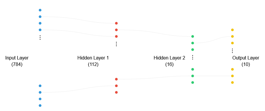
Now for the fun part - building our network from scratch! I thought it would be neat to start with 2 hidden layers:
- Input layer: 784 neurons (one for each pixel)
- First hidden layer: 112 neurons
- Second hidden layer: 16 neurons
- Output layer: 10 neurons (one for each digit)
The Building Blocks
1. Initialization (__init__)
The network starts life with random weights and biases. Each connection between neurons gets a random weight between -0.5 and 0.5. Why? We want to start with small random values to break symmetry and allow the network to learn different patterns.
Initializing the network with weights and biases
class My_Neural_Network:
    def __init__(self, layer_sizes):
    self.sizes = layer_sizes
    self.num_layers = len(layer_sizes)
    self.weights = []
    self.biases = []

    for i in range(len(self.sizes)-1):
    layer_weights = []
    for destination_neuron in range(self.sizes[i+1]):
        neuron_weights = []
        for source_neuron in range(self.sizes[i]):
            weight = (random.random() - 0.5)
            neuron_weights.append(weight)
        layer_weights.append(neuron_weights)
    self.weights.append(layer_weights)

    #Start with bias=1 for next layer
    layer_biases = [1.0 for _ in range(self.sizes[i+1])]
    self.biases.append(layer_biases)
2. Activation Function (sigmoid)
We use the sigmoid function to squash any input into a value between 0 and 1. It's like a smooth step function:
- Very negative inputs → output close to 0
- Very positive inputs → output close to 1
- Inputs around 0 → gradual transition
Defining our activation function
def sigmoid(self, x):
    # Handle extreme values to prevent overflow
    if x < -700:
        return 0.0
    elif x > 700:
        return 1.0
    return 1.0/(1.0 + math.exp(-x))

def sigmoid_derivative(self, x):
    # This is the derivative of sigmoid: sigmoid(x) * (1 - sigmoid(x))
    return self.sigmoid(x) * (1 - self.sigmoid(x))
Why do we check for ±700? The sigmoid function involves e^(-x), and Python's math.exp() can overflow with large values. Since sigmoid(700) is already extremely close to 1 (and sigmoid(-700) to 0), we can safely clamp values beyond these bounds.
3. Forward Propagation (feedforward)
This is how our network makes predictions. Data flows through the layers like this:
Defining how our neural network spits an output for a given input
def feedforward(self, inputs):
    """
    Push data through the network to get predictions. Returns:
    1. Activations - neuron outputs at each layer
    2. Weighted sums - the values before sigmoid activation (needed for backprop)
    """
    current_values = inputs
    all_activations = [inputs]  # Store all layer outputs
    all_weighted_sums = []      # Store all pre-activation values

    # Process each layer
    for layer_weights, layer_biases in zip(self.weights, self.biases):
    # Calculate weighted sums for each neuron in current layer
    weighted_sums = []
    for weights, bias in zip(layer_weights, layer_biases):
        # For each neuron:
        # 1. Multiply each input by its weight
        # 2. Sum all weighted inputs
        # 3. Add the bias
        total = sum(w * a for w, a in zip(weights, current_values))
        weighted_sums.append(total + bias)

    # Store pre-activation values for backprop
    all_weighted_sums.append(weighted_sums)

    # Apply sigmoid activation to get neuron outputs
    current_values = [self.sigmoid(z) for z in weighted_sums]
    all_activations.append(current_values)

    return all_activations, all_weighted_sums
With a given input vector, here's what happens in the forward pass:
- We start with our input layer
- For each subsequent layer:
- Each neuron calculates its weighted sum (z = w₁a₁ + w₂a₂ + ... + b)
- We store these weighted sums (we'll need them for backpropagation)
- Apply the sigmoid function to each weighted sum to get neuron outputs
- These outputs become the inputs for the next layer
- We keep track of ALL values because backpropagation needs them:
- all_activations: Output of each layer (after sigmoid)
- all_weighted_sums: Values before sigmoid (needed for derivatives)
The zip(layer_weights, layer_biases) lets us process corresponding weights and biases together. For each neuron, we compute its output in two steps:
- Weighted sum: Multiply each input by its weight and sum (plus bias)
- Activation: Pass this sum through sigmoid to get output between 0 and 1
4. Backpropagation
This is where the magic happens. Backpropagation is how our network learns from its mistakes. Here's the complete implementation:
Backpropagation - teaching our NN to learn
def backpropagate(self, training_example, label):
    """
    1. Calculate the network's error
    2. Determine how each weight contributed to that error
    3. Return gradients for weights and biases
    """
    # First, do a forward pass to get all intermediate values
    activations, weighted_sums = self.feedforward(training_example)

    # Initialize gradients as zero
    weight_gradients = [[[0.0 for _ in range(len(w_row))]
                    for w_row in layer]
                    for layer in self.weights]
    bias_gradients = [[0.0 for _ in range(len(b))]
                for b in self.biases]

    # Calculate error at the output layer
    # Error = (actual - target) * sigmoid_derivative(output)
    output_error = [a - t for a, t in zip(activations[-1], label)]
    layer_error = [err * self.sigmoid_derivative(a)
            for err, a in zip(output_error, activations[-1])]

    # Save gradients for output layer
    bias_gradients[-1] = layer_error
    for i, error in enumerate(layer_error):
    for j, activation in enumerate(activations[-2]):
        weight_gradients[-1][i][j] = error * activation

    # Backpropagate error through earlier layers
    for layer in range(2, self.num_layers):
    layer_error_new = []

    # For each neuron in current layer
    for j in range(len(self.weights[-layer])):
        # Calculate error based on next layer's error
        error = 0.0
        for k in range(len(layer_error)):
            error += self.weights[-layer+1][k][j] * layer_error[k]
        error *= self.sigmoid_derivative(activations[-layer][j])
        layer_error_new.append(error)

    layer_error = layer_error_new

    # Save gradients
    bias_gradients[-layer] = layer_error
    for i, error in enumerate(layer_error):
        for j, activation in enumerate(activations[-layer-1]):
            layer_index = len(self.weights) - layer
            weight_gradients[layer_index][i][j] = error * activation

    return weight_gradients, bias_gradients
Let's walk through this carefully. For a detailed, mathematical understanding of backpropagation, I can't recommend Matt Mazur's post enough. Brilliant piece of writing.
Step 1: Output Layer Error
For the output layer, calculating the error is reasonably easy:
- Error = (actual output - desired output) * sigmoid_derivative(output)
- We multiply by sigmoid_derivative because we need to account for how the sigmoid function would change with small adjustments. See the link above for a step by step reasoning for how we got to this equation.
- This tells us how much each output neuron contributed to the error.
Step 2: Hidden Layer Error
For hidden layers, it's more of the same. We need to:
- Take each neuron in the current layer
- Look at ALL connections to the next layer
- Sum up (next layer's error * connection weight) for each connection
- Multiply by sigmoid_derivative of the current neuron's output
This is the chain rule in action: we're calculating how much each hidden neuron contributed to the final error by looking at all paths from that neuron to the output.
Step 3: Weight Gradients
For each weight, its gradient is:
gradient = (error of receiving neuron) * (activation of sending neuron)
This makes intuitive sense. If the receiving neuron had a large error, we want to change its weights more. If the sending neuron had a large activation, it contributed more to the error. If either value is small, the weight didn't contribute much to the error.
Step 4: Using the Gradients
These gradients tell us how to adjust each weight to reduce the error:
- Positive gradient → weight contributed to positive error → decrease weight
- Negative gradient → weight contributed to negative error → increase weight
- The learning rate determines how big these adjustments are. This is one of the hyperparameters we set during the training.
5. Training
The training process ties everything together. One thing to note is that MNIST is a solved problem now, with the best solutions achieving >99% accuracy. Through countless experiments, researchers have discovered optimal architectures and hyperparameters. Our implementation ignores these guidelines for the sake of learning, and consequently achieves a more modest accuracy.
Let's look at the three main approaches to training neural networks:
- Stochastic Gradient Descent (SGD): Updates weights after every single training example. Very fast per update but produces noisy learning. Can zigzag toward the solution due to frequent updates and is sensitive to outliers. Good for online learning where data comes in real-time.
- Full Batch Gradient Descent: Processes the entire training dataset before making any weight updates. Very stable since it averages over all examples, but requires lots of memory and can only make one update per epoch. Often too computationally expensive for large datasets and more likely to get stuck in local minima.
- Mini-batch Gradient Descent (our approach): Processes a small batch of examples (in our case, 32) before updating. This hits a sweet spot - more stable than SGD but still allows frequent updates, less memory-intensive than full batch.
We use mini-batch gradient descent with a batch size of 32. Here's how the training works:
Training - updating mini batches -> training on each mini batch -> predicting on the validation set -> evaluating performance
def update_mini_batch(self, mini_batch, learning_rate):
    #Update network weights using a small batch of shuffled training data

    #Initialize gradient sums as zero

    weight_sums = [[[0.0 for _ in range(len(w_row))]
                    for w_row in layer]
                    for layer in self.weights]

    bias_sums = [[0.0 for _ in range(len(b))]
                    for b in self.biases]

    #Calculate gradients for each training example
    for inputs, label in mini_batch:
        weight_gradients, bias_gradients = self.backpropagate(inputs, label)

        #Add to sums
        for layer in range(len(weight_sums)):
            for i in range(len(weight_sums[layer])):
                for j in range(len(weight_sums[layer][i])):
                    weight_sums[layer][i][j] += weight_gradients[layer][i][j]

        for layer in range(len(bias_sums)):
            for i in range(len(bias_sums[layer])):
                bias_sums[layer][i] += bias_gradients[layer][i]

    # Update weights and biases using average gradients
    batch_size = len(mini_batch)
    for layer in range(len(self.weights)):
        for i in range(len(self.weights[layer])):
            for j in range(len(self.weights[layer][i])):
                self.weights[layer][i][j] -= (learning_rate/batch_size) * weight_sums[layer][i][j]

        for i in range(len(self.biases[layer])):
            self.biases[layer][i] -= (learning_rate/batch_size) * bias_sums[layer][i]

def train(self, training_data, epochs, mini_batch_size, learning_rate):
    #Train the network on batches of data
    n = len(training_data)

    for epoch in range(epochs):
        #Shuffle the training data
        random.shuffle(training_data)

        #Create mini-batches
        mini_batches = [
            training_data[k:k+ mini_batch_size]
            for k in range(0, n , mini_batch_size)
        ]

        #Train on each mini-batch
        print(f" Epoch {epoch + 1}: Training on {len(mini_batches)} batches")
        for i, mini_batch in enumerate(mini_batches):
            if i % 100 == 0:
                #Show progress every 100 batches
                print(f" Batch {i}/{len(mini_batches)}")
            self.update_mini_batch(mini_batch, learning_rate)

        #Calculate and show accuracy
        accuracy = self.evaluate(validation_data)
        print(f"Epoch {epoch+1}: {accuracy:.2f}% accuracy")

def predict(self, inputs):
    #Get network's prediction (0-9) for an input
    activations, _ = self.feedforward(inputs)
    output = activations[-1]
    return output.index(max(output))

def evaluate(self, test_data):
    #Calcuate accuracy on test data
    correct = 0
    total = len(test_data)

    for inputs, label in test_data:
        prediction = self.predict(inputs)
        actual = list(label).index(1)
        #We are bringing the label back from one-hot-encoded to a numeric form
        if prediction == actual:
            correct += 1

    return (correct/total)*100
The Results
After 10 epochs of training, our network achieves around 75% accuracy on the validation set and 76% on the testing set. This is decidedly basic compared to modern deep learning models (which hit 99%+), but remember - we built this using only basic Python operations! No optimized matrix operations, no GPU acceleration, no fancy optimizers.
Key Takeaways
Building a neural network from scratch teaches us several important lessons:
- Neural networks aren't magic - they're just lots of simple math operations chained together
- The basic principles (forward pass, backprop, gradient descent) haven't changed since the 1980s
- Modern frameworks abstract away these details, but understanding them helps debug and optimize networks
- Even a simple network can learn meaningful patterns
Want to understand backpropagation in even more detail? Check out this excellent step-by-step guide that helped me grasp the concepts.
The complete code with detailed comments is available in this GitHub repo. Feel free to experiment with different architectures, learning rates, and batch sizes!